What is The Phillips Curve

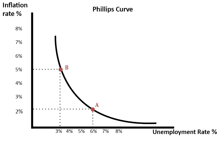
Reducing inflation is often thought to cause a temporary rise in unemployment. The curve that illustrates this tradeoff between inflation and unemployment is called the Phillips curve, named after the economist who first examined this relationship.

The Phillips curve remains a controversial topic among economists, but most economists today accept the idea that there is a short-run tradeoff between inflation and unemployment.

This simply means that, over a period of a year or two, many economic policies push inflation and unemployment in opposite directions.

Table of Contents

1. A trade-off between Inflation and Employment
2. Aggregate Demand, Supply, and the Phillips curve
3. Phillips Curve Equation
4. Phillips Curve in Long Run

Short-run tradeoff

According to a common explanation, short-term tradeoff, arises because some prices are slow to adjust.

Suppose — for example —

To curb the Economy, the government reduces the quantity of money in the economy. In the long run, the only result of this policy change will be a fall in the overall level of prices.

Yet not all prices will adjust immediately.

It may take several years before all firms issue new catalogs, all unions make wage concessions, and all restaurants print new menus. That is, prices are said to be sticky in the short run.

Because prices are sticky, various types of government policy have short-run effects that differ from their long-run effects.

When the government reduces the quantity of money, for instance, it reduces the total amount that people spend. Lower spending and already high prices reduce the number of goods and services that the company sells.

Lower sales, in turn, cause firms to lay off workers. Thus, the reduction in the quantity of money raises unemployment temporarily until prices have fully adjusted to the change.

The tradeoff between inflation and unemployment is only temporary, but it can last for several years.

The Phillips curve is, therefore, crucial for understanding many developments in the economy. In particular, policymakers can exploit this tradeoff using various policy instruments.

By changing the amount that the government spends, the amount it taxes, and the amount of money it prints, policymakers can, in the short run, influence the combination of inflation and unemployment that the economy experiences.

Because these instruments of monetary and fiscal policy are potentially so powerful, how policymakers should use these instruments to control the economy, if at all, is a subject of continuing debate.

AGGREGATE DEMAND, AGGREGATE SUPPLY, AND THE PHILLIPS CURVE

The model of aggregate demand and aggregate supply provides an easy explanation for the menu of possible outcomes described by the Phillips curve.

The Phillips curve simply shows the combinations of inflation and unemployment that arise in the short run as shifts in the aggregate-demand curve move the economy along the short-run aggregate supply curve.

An increase in the aggregate demand for goods and services leads, in the short run, to a larger output of goods and services and a higher price level.

The larger output means greater employment and, thus, a lower rate of unemployment.

In addition, whatever the previous year’s price level happens to be, the higher the price level in the current year, the higher the rate of inflation.

Thus, shifts in aggregate demand push inflation and unemployment in opposite directions in the short run—a relationship illustrated by the Phillips curve.

To see more fully how this works, let’s consider an example.

To keep the numbers simple, imagine that the price level (as measured, for instance, by the consumer price index) equals 100 in the year 2000

There are two possible outcomes that might occur in the year 2001.

In this Graph, we can see the implications for output and the price level in the year 2001. If the aggregate demand for goods and services is relatively low, the economy experiences outcome A.

By contrast, if aggregate demand is relatively high, the economy experiences outcome B. Where Output is 8,000, and the price level is 106.

Thus, higher aggregate demand moves the economy to equilibrium with higher output and a higher price level.

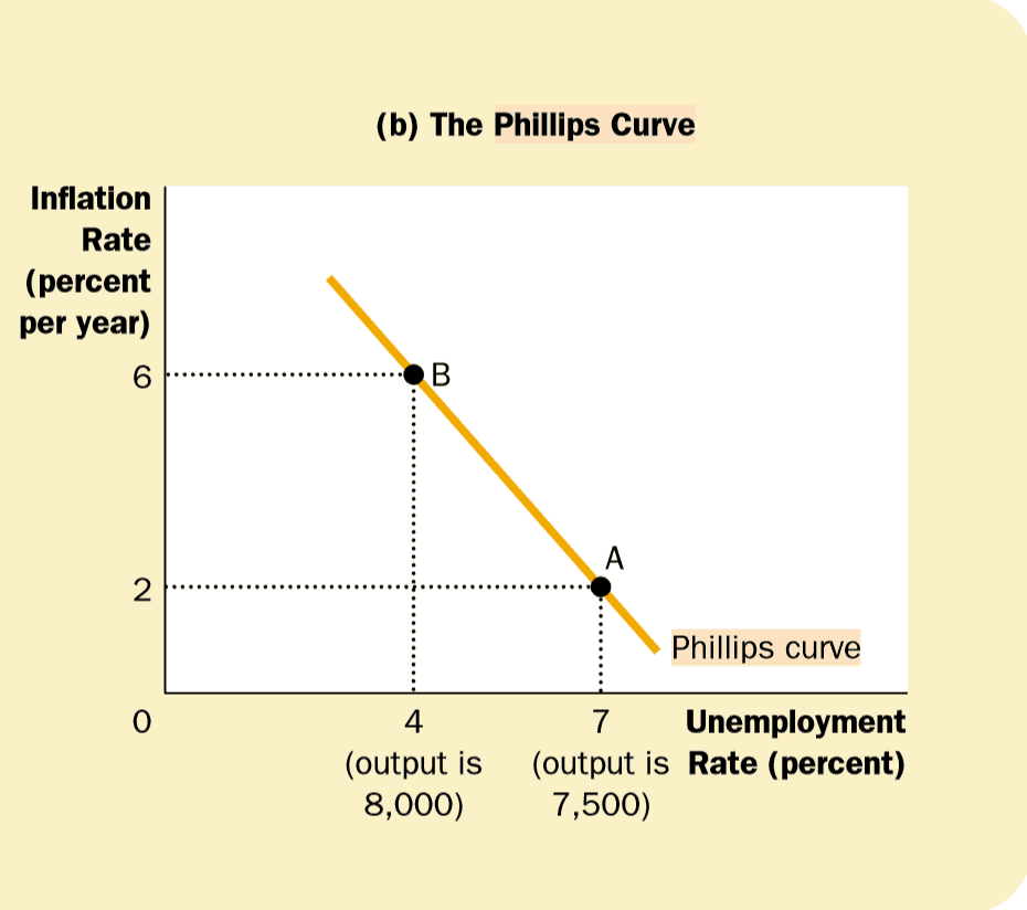
In Phillip curve graph (Graph 2),

we can see what these two possible outcomes mean for unemployment and inflation.

Because firms need more workers when they produce a greater output of goods and services, unemployment is lower in outcome B than in outcome A.

In this example, when output rises from 7,500 to 8,000, unemployment falls from 7 percent to 4 percent.

Moreover, because the price level is higher at outcome B than at outcome A, the inflation rate (the percentage change in the price level from the previous year) is also higher.

In particular, since the price level was 100 in the year 2000, outcome A has an inflation rate of 2 percent, and outcome B has an inflation rate of 6 percent.

Thus, we can compare the two possible outcomes for the economy either in terms of output and the price level (using the model of aggregate demand and aggregate supply) or in terms of unemployment and inflation (using the Phillips curve).

Monetary and fiscal policy can shift the aggregate demand curve. Therefore, the monetary and fiscal policy can move the economy along the Phillips curve.

Increases in the money supply increases in government spending or cuts in taxes expand aggregate demand and move the economy to a point on the Phillips curve with lower unemployment and higher inflation.

Decreases in the money supply, cuts in government spending, or increases in taxes contract aggregate demand and move the economy to a point on the Phillips curve with lower inflation and higher unemployment.

In this sense, the Phillips curve offers policymakers a menu of combinations of inflation and unemployment.

Simple Phillips Curve Equation

U = -h* (unemployment – u_n ) 

π = -h* (u – u_n )

This simple Phillips curve is generally written with inflation as a function of the unemployment rate and the hypothetical unemployment rate that would exist if inflation were equal to zero.

Typically, the inflation rate is represented by pi and the unemployment rate is represented by u.

Theh in the phillips curve equation is a positive constant that guarantees that the Phillips curve slopes downwards, and the un is the “natural” rate of unemployment that would result if inflation were equal to zero. (This is not to be confused with the NAIRU, which is the unemployment rate that results with non-accelerating, or constant, inflation).

Inflation and unemployment can be recorded either as numbers or as the percentage, so it’s crucial to determine from circumstances that are appropriate. For example, an unemployment rate of 7 percent could either be written as 7% or 0.07.

Phillips Curve in Long Run

There is no tradeoff between inflation and unemployment in the long run.

Growth in the money supply determines the inflation rate. Regardless of the inflation rate, the unemployment rate gravitates toward its natural rate.

As a result, the long-run Phillips curve is vertical.

As a result of this shift, the long-run equilibrium moves from point A to point B. The price level rises from P1 to P2, but because the aggregate-supply curve is vertical, output remains the same.

Rapid growth in the money supply raises the inflation rate by moving the economy from point A to point B. But because the Phillips curve is vertical, the rate of unemployment is the same at these two points.

Thus, the vertical long-run aggregate supply curve and the vertical long-run Phillips curve both imply that monetary policy influences nominal variables (the price level and the inflation rate) but not real variables (output and unemployment).

Regardless of the monetary policy pursued by the Fed(Government), output and unemployment are, in the long run, at their natural rates